The following code creates visualizations for diagnostic related
information. The main difficulty of these visualizations was getting
diagnostic variables correctly coded so there was not overlap or double
acounting for conditions.
Create Diagnosis Variables
Mothership<-Mothership %>%
  mutate(
          # Mood Disorders
                     Mood_D = as.factor(
                      ifelse(
                        MDD_P ==1 | Bipolar1_P == 1 | Bipolar2_P == 1 | Dysthymia_P == 1, 1, 0)),
          # Anxiety Disorders
                    Anxiety_D = as.factor(
                      ifelse(
                        GAD_P ==1 | Panic_P == 1 | PanicAgor_P == 1 | Agoraphobia_P == 1 |
                        Social_P == 1 | Specific_P == 1, 1, 0)),
          # Obsessive Compusive Disorders
                #OCD_P is for current OCD
                OCD_P = as.factor(OCD_P),
          # Personality Disorders
                #BPD_P is for current BPD
                BPD_P = as.factor(BPD_P),
          # Substance Use Disorders
                    Substance_D = as.factor(
                      ifelse(
                        Alcohol_P == 1 | Drug_P ==1, 1, 0)),
          # Trauma or stresor related disorders
                    Trauma_D = as.factor(
                      ifelse(PTSD_P == 1 | Adjustment_P ==1, 1,0)),
          # Psychotic Disorders
                    Psychotic_D = as.factor(
                      ifelse(
                        Schiz_P == 1 | Schizaff_P == 1,1,0)),
            # Eating Disorders
                    Eating_D = as.factor(
                      ifelse(
                        Anorex_P == 1 | Bulim_P == 1 | Binge_P == 1, 1,0)),
            # Somatic Disroders
                    Somatic_D = as.factor(
                      ifelse(
                        Somat_P == 1 | UndiffSoma_P == 1| Hypochondriasis_P ==1,
                        1,0)),
                    Disorder_Type = as.factor(
                      ifelse(Anxiety_D == 1, "Anxiety",
                      ifelse(OCD_P == 1, "OCD",
                      ifelse(BPD_P == 1, "BPD",
                      ifelse(Substance_D == 1, "Substance Use",
                      ifelse(Trauma_D == 1, "Trauma",
                      ifelse(Mood_D == 1, "Mood",
                      ifelse(Psychotic_D == 1, "Psychotic",
                      ifelse(Eating_D == 1, "Eating",
                      ifelse(Somatic_D == 1, "Somatic", NA
                      )))))))))),
                    Disorder_treat = as.factor(
                      ifelse(Anxiety_D == 1, "Anxiety",
                      ifelse(BPD_P == 1, "BPD",
                      ifelse(Trauma_D == 1, "Trauma",
                      ifelse(Mood_D == 1, "Mood",
                      NA
                      ))))),
                  Anxiety_C =  as.factor(
                    ifelse( GAD_P !=1 & GAD_C ==1 |
                        Panic_P != 1 & Panic_C == 1 |
                        PanicAgor_P != 1 & PanicAgor_C == 1 |
                        Agoraphobia_P != 1 & Agoraphobia_C == 1 |
                        Social_P != 1 & Social_C == 1 |
                        Specific_P != 1 & Specific_C == 1, 1, 0)),
                  Mood_C =  as.factor(
                    ifelse( MDD_P != 1 & MDD_C == 1 |
                        Bipolar1_P != 1 & Bipolar1_C == 1 |
                        Bipolar2_P != 1 &  Bipolar2_C == 1 |
                        Dysthymia_P != 1 & Dysthymia_C == 1 , 1, 0)),
                  Substance_C = as.factor(
                    ifelse(Alcohol_P != 1 & Alcohol_C == 1 |
                        Drug_P != 1 & Drug_C ==1, 1, 0)),
                  Trauma_C = as.factor(
                    ifelse(PTSD_P != 1 & PTSD_C == 1 |
                        Adjustment_P != 1 & Adjustment_C ==1, 1,0)),
                  Psychotic_C = as.factor(
                    ifelse(Schiz_P != 1 & Schiz_C == 1 |
                        Schizaff_P != 1 & Schizaff_C == 1,1,0)),
                  Eating_C = as.factor(
                    ifelse(Anorex_P != 1 & Anorex_C == 1 |
                        Bulim_P != 1 & Bulim_C == 1 |
                        Binge_P != 1 & Binge_C == 1, 1,0)),
                  Somatic_C = as.factor(
                    ifelse(Somat_P != 1 & Somat_C == 1 |
                        UndiffSoma_P != 1 & UndiffSoma_C == 1 |
                        Hypochondriasis_P != 1 &  Hypochondriasis_C == 1, 1,0)),
                  OCD_Co_C = as.factor(
                    ifelse(OCD_P != 1 & OCD_C == 1,1,0)),
                  BPD_Co_C = as.factor(
                    ifelse(BPD_P != 1 & BPD_C ==1,1,0)),
                  No_Co = as.factor(
                    ifelse(BPD_Co_C == 0 &
                           OCD_Co_C == 0 &
                           Somatic_C == 0 &
                           Eating_C == 0 &
                           Psychotic_C == 0 &
                           Trauma_C == 0 &
                           Substance_C == 0 &
                           Mood_C == 0 &
                           Anxiety_C == 0, 1,0)),
                  Other_Co = as.factor(
                    ifelse(OCD_Co_C == 1 &
                           Somatic_C == 0 &
                           Eating_C == 0 &
                           Psychotic_C == 0,1,0)),

          #emotional disorders
                  Emotional_dis = as.factor(
                    ifelse(Anxiety_D == 1 | OCD_P == 1 | Trauma_D == 1 |
                           Mood_D == 1, "Emotional Disorder", "Other Disorder")),
                  Co_Anx = as.factor(
                        ifelse(Anxiety_D == 1 & Mood_C == 1 |
                                Anxiety_D == 1 & OCD_C == 1 |
                                Anxiety_D == 1 & BPD_C == 1 |
                                Anxiety_D == 1 & Substance_C == 1 |
                                Anxiety_D == 1 & Trauma_C == 1 |
                                Anxiety_D == 1 & Eating_C ==1 |
                                Anxiety_D == 1 & Psychotic_C ==1 |
                                Anxiety_D == 1 & Somatic_C ==1, 1, 0)),
                  Co_Mood = as.factor(
                        ifelse(Mood_D == 1 & Anxiety_C == 1 |
                                Mood_D == 1 & OCD_C == 1 |
                                Mood_D == 1 & BPD_C == 1 |
                                Mood_D == 1 & Substance_C == 1 |
                                Mood_D == 1 & Trauma_C == 1 |
                                Mood_D == 1 & Eating_C ==1 |
                                Mood_D == 1 & Psychotic_C ==1 |
                                Mood_D == 1 & Somatic_C ==1 , 1, 0)),
                  Co_OCD = as.factor(
                        ifelse(OCD_C == 1 & Anxiety_C == 1 |
                                OCD_C == 1 & Mood_C == 1 |
                                OCD_C == 1 & BPD_C == 1 |
                                OCD_C == 1 & Substance_C == 1 |
                                OCD_C == 1 & Trauma_C == 1 |
                                OCD_C == 1 & Eating_C ==1 |
                                OCD_C == 1 & Psychotic_C ==1 |
                                OCD_C == 1 & Somatic_C ==1, 1, 0)),
                  CO_BPD = as.factor(
                        ifelse(BPD_C == 1 & Anxiety_C == 1 |
                                BPD_C == 1 & Mood_C == 1 |
                                BPD_C == 1 & OCD_C == 1 |
                                BPD_C == 1 & Substance_C == 1 |
                                BPD_C == 1 & Trauma_C == 1 |
                                BPD_C == 1 & Eating_C ==1 |
                                BPD_C == 1 & Psychotic_C ==1 |
                                BPD_C == 1 & Somatic_C ==1 , 1, 0)),
                  CO_Psychotic = as.factor(
                       ifelse(Psychotic_D == 1 & Mood_C == 1 |
                                Psychotic_D == 1 & OCD_C == 1 |
                                Psychotic_D == 1 & BPD_C == 1 |
                                Psychotic_D == 1 & Substance_C == 1 |
                                Psychotic_D == 1 & Trauma_C == 1 |
                                Psychotic_D == 1 & Eating_C ==1 |
                                Psychotic_D == 1 & Anxiety_C ==1 |
                                Psychotic_D == 1 & Somatic_C ==1, 1, 0)),
                  CO_Eating = as.factor(
                      ifelse(Eating_D == 1 & Mood_C == 1 |
                                Eating_D == 1 & OCD_C == 1 |
                                Eating_D == 1 & BPD_C == 1 |
                                Eating_D == 1 & Substance_C == 1 |
                                Eating_D == 1 & Trauma_C == 1 |
                                Eating_D == 1 & Psychotic_C ==1 |
                                Eating_D == 1 & Anxiety_C ==1 |
                                Eating_D == 1 & Somatic_C ==1, 1, 0)),
                  CO_Somatic =  as.factor(
                       ifelse(Somatic_D == 1 & Mood_C == 1 |
                                Somatic_D == 1 & OCD_C == 1 |
                                Somatic_D == 1 & BPD_C == 1 |
                                Somatic_D == 1 & Substance_C == 1 |
                                Somatic_D == 1 & Trauma_C == 1 |
                                Somatic_D == 1 & Eating_C ==1 |
                                Somatic_D == 1 & Anxiety_C ==1 |
                                Somatic_D == 1 & Psychotic_C ==1, 1, 0)))

##### df for plots

# df without NAs in date and disorder type
Mothership_Diag <- Mothership %>%
  filter(!is.na(Disorder_Type))%>%
  filter(!is.na(TxYear))

Mothership_Diag_treat <- Mothership %>%
  filter(!is.na(Disorder_treat))%>%
  filter(!is.na(TxYear))
# df with and without depression
No_depressy <- Mothership_Diag %>%
  filter(Disorder_Type != "Mood")

view(Mothership)
Number of Disorders Treated Over Time
All Disorders
# Libraries
library(ggplot2)
#install.packages("hrbrthemes")
library(hrbrthemes)
library(dplyr)
library(tidyr)
library(viridis)
# Stacked
ggplot(data=subset(Mothership_Diag, !is.na(Disorder_Type)),
mapping= aes(x=TxYear, y = stat(count),
group=Disorder_Type, fill=Disorder_Type)) +
geom_density(adjust=1.5,alpha=.4,position="fill") +
theme(axis.text.x = element_text(angle = 45,hjust = 1))+
theme(panel.grid.major.y = element_line(color = "grey",size = 0.5,linetype = 2))+
xlab("Treatment Year") +
theme(panel.background=NULL) +
facet_wrap(~Emotional_dis)+
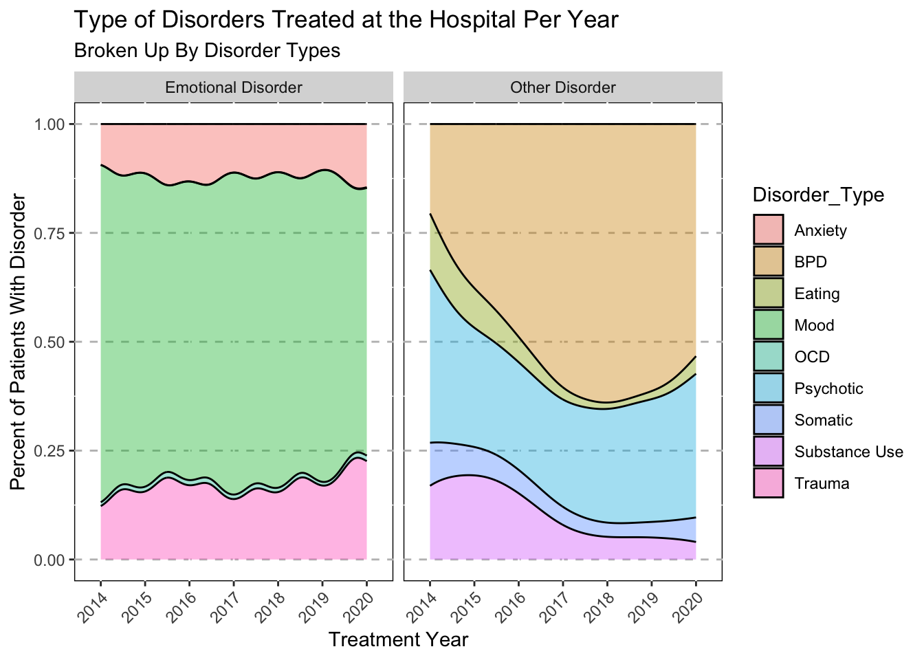
labs(
title = "Type of Disorders Treated at the Hospital Per Year",
subtitle = "Broken Up By Disorder Types") +
xlab("Treatment Year") +
ylab("Percent of Patients With Disorder")
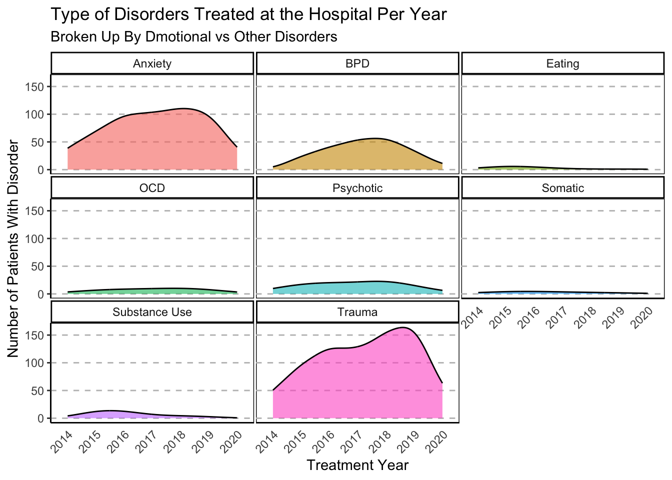
# Broken up by disorder.
ggplot(data=subset(Mothership_Diag, !is.na(Disorder_Type)),
mapping= aes(x=TxYear,y = stat(count),
group=Disorder_Type, fill=Disorder_Type)) +
geom_density(adjust=1.5,alpha=.6) +
facet_wrap(~Disorder_Type)+
theme_classic()+
theme(
panel.grid.major.y = element_line(color = "grey",size = 0.5,linetype = 2),
axis.text.x = element_text(angle = 45,hjust = 1),
legend.position="none",
panel.spacing = unit(0.1, "lines"),
axis.ticks.x=element_blank(),
panel.background=NULL) +
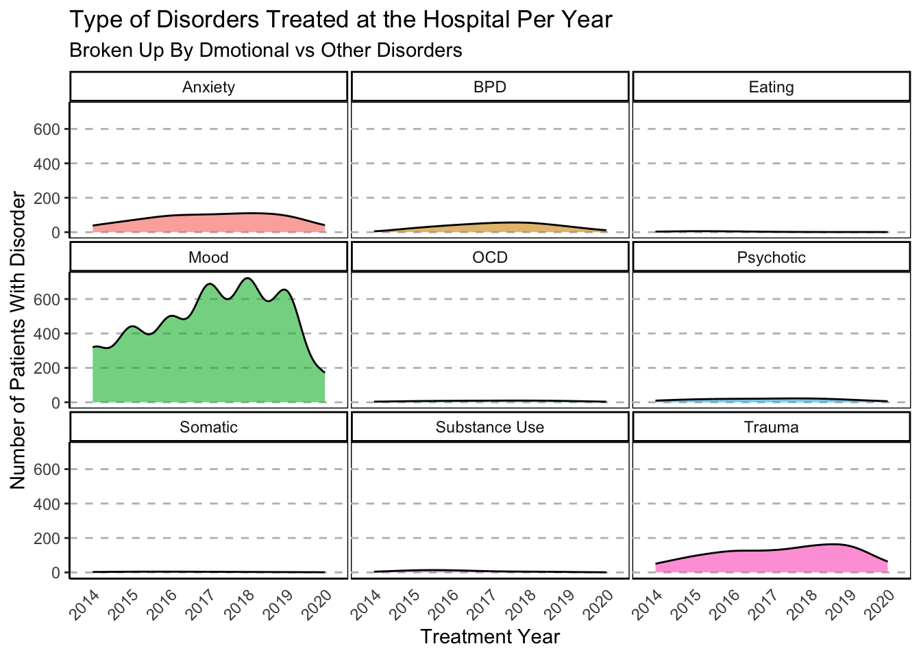
labs(
title = "Type of Disorders Treated at the Hospital Per Year",
subtitle = "Broken Up By Dmotional vs Other Disorders") +
xlab("Treatment Year") +
ylab("Number of Patients With Disorder")
 ### Excluding Mood Disorders
# without depression
ggplot(data=subset(No_depressy, !is.na(Disorder_Type)),
    mapping= aes(x=TxYear,y = stat(count),
                 group=Disorder_Type, fill=Disorder_Type)) +
  geom_density(adjust=1.5,alpha=.6) +
  facet_wrap(~Disorder_Type)+
  theme_classic()+
    theme(
      panel.grid.major.y = element_line(color = "grey",size = 0.5,linetype = 2),
      axis.text.x = element_text(angle = 45,hjust = 1),
      legend.position="none",
      panel.spacing = unit(0.1, "lines"),
      axis.ticks.x=element_blank(),
      panel.background=NULL) +
  labs(
    title = "Type of Disorders Treated at the Hospital Per Year",
    subtitle = "Broken Up By Dmotional vs Other Disorders") +
    xlab("Treatment Year") +
    ylab("Number of Patients With Disorder")
Amount of Disorder Type Treated
Grouped into DSM chapter subtypes (e.g., Mood Disorder = Major
Depressive Disorder, Bipolar 1 & 2, etc.)
Amount of Primary Diagnoses
# Disorder Type
ggplot(data = subset(Mothership_Diag, !is.na(Disorder_Type)),mapping = aes(x = Disorder_Type, fill=Disorder_Type))+
  geom_bar()+
  ggtitle("Frequency of Psychiatric Disorder Subtypes") +
  theme(axis.text.x = element_text(angle = 45,hjust = 1),
        legend.position = "none")+
  xlab("Psychiatric Disorder Subtype")+
  theme(panel.grid.major.x = element_line(color = "grey",size = 0.5,linetype = 2))+
  theme(panel.background=NULL)+
  scale_y_continuous(name = "Frequency",limits=c(0,3500))+
  coord_flip()
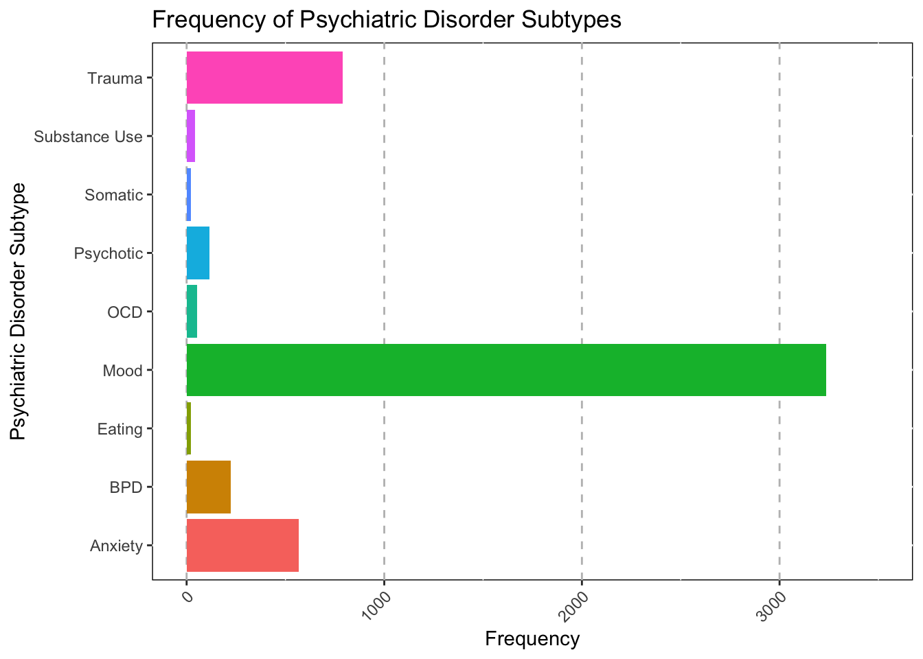
As you can see, the main disorder type in the hospital is mood
realted disorders. This shouldn’t be supprising as many indiviudals with
suicidality (A common hospitalization issue) will meet criteria for a
mood disorder.
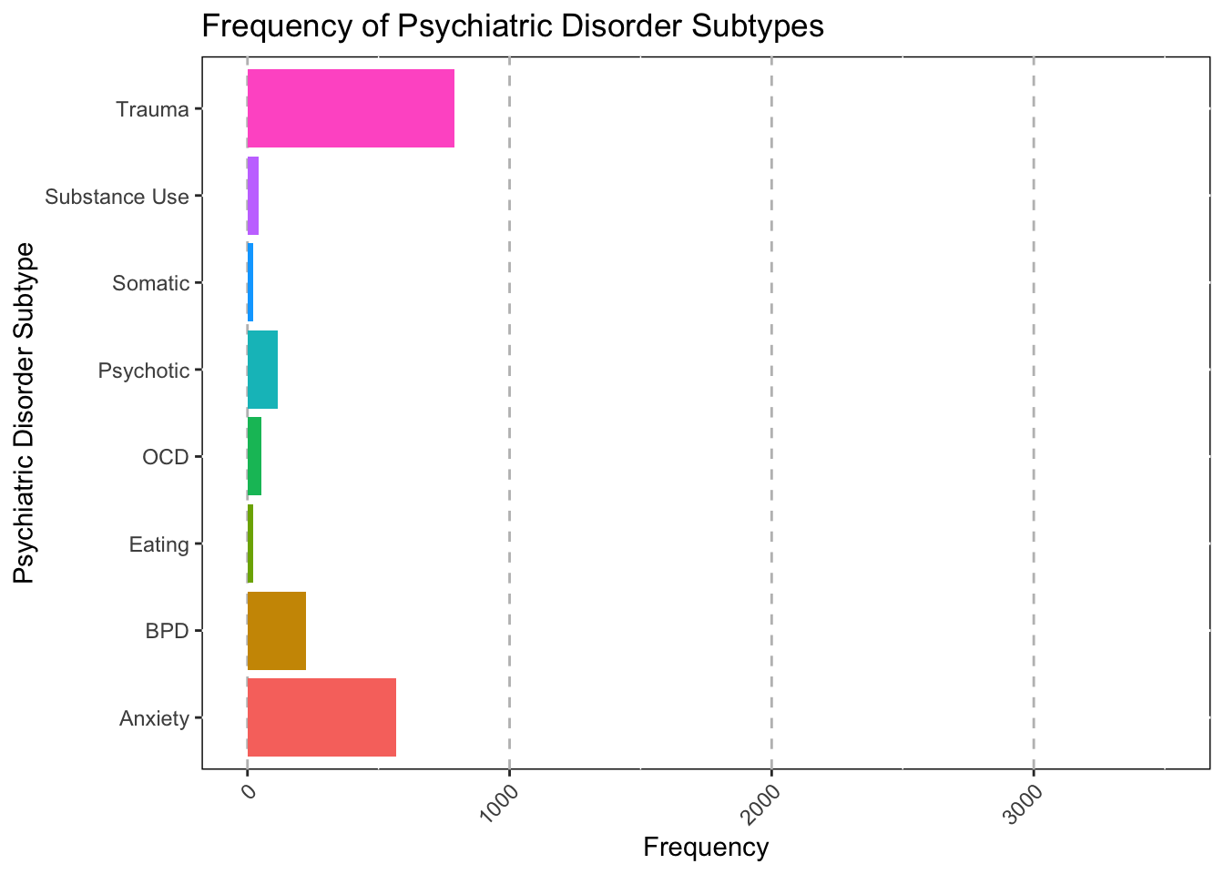
Excluding Mood Disorders
# Disorder Type (Without Depression)
ggplot(data = subset(No_depressy, !is.na(Disorder_Type)),mapping = aes(x = Disorder_Type, fill=Disorder_Type))+
  geom_bar()+
  ggtitle("Frequency of Psychiatric Disorder Subtypes") +
  theme(axis.text.x = element_text(angle = 45,hjust = 1),
        legend.position = "none")+
  xlab("Psychiatric Disorder Subtype")+
  theme(panel.grid.major.x = element_line(color = "grey",size = 0.5,linetype = 2))+
  theme(panel.background=NULL)+
  scale_y_continuous(name = "Frequency",limits=c(0,3500))+
  coord_flip()
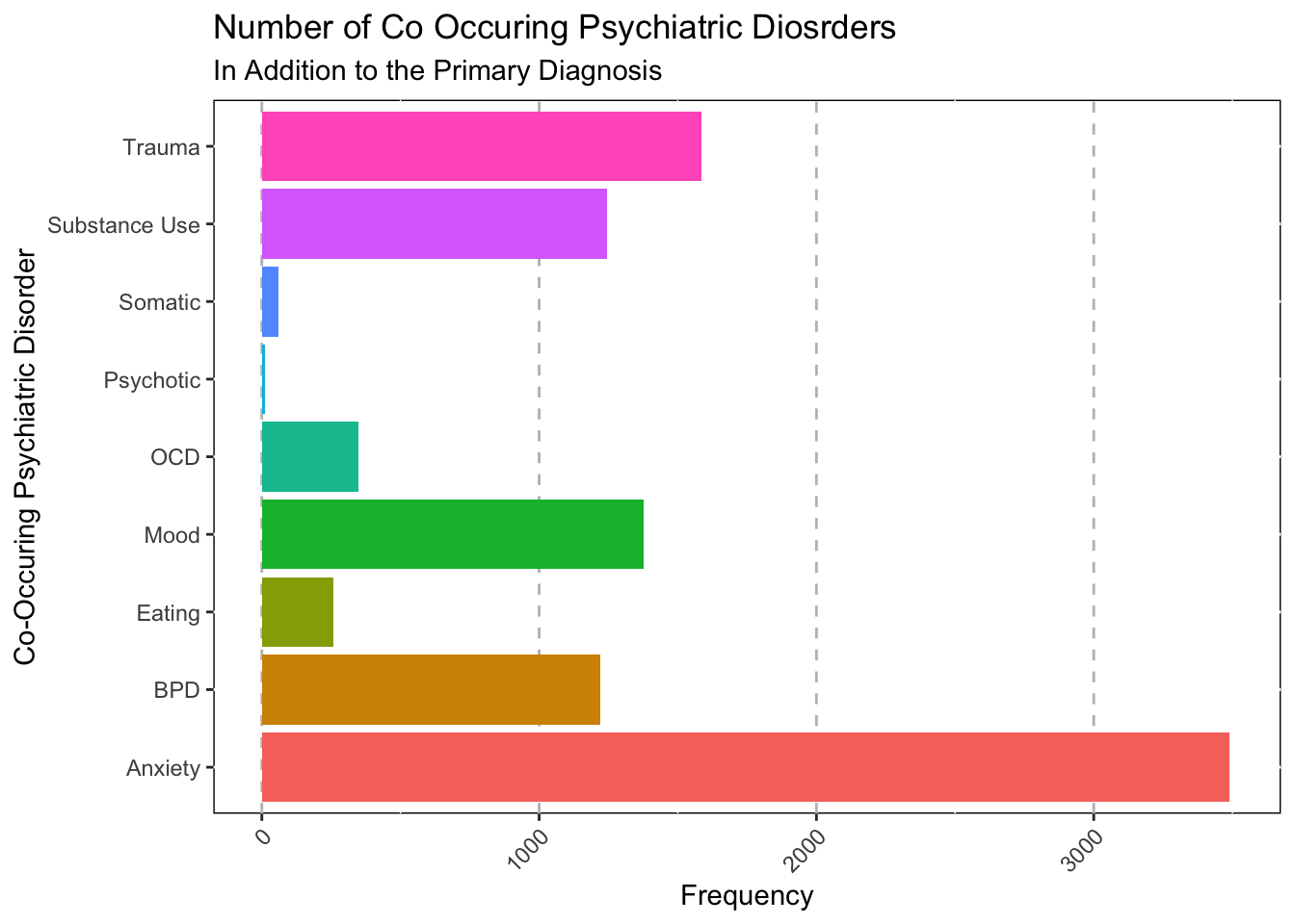
Number of Co-occuring Disorders
The following visualization looks at the number of disorders people
had, but wasn’t the main reason they attended the hospital, or their
“main” diagnosis.
Mothership_Current_Long <- Mothership %>%
  pivot_longer(
    cols=c(Anxiety_C, Mood_C, Substance_C, Trauma_C, Psychotic_C, Eating_C,  Somatic_C, OCD_Co_C, BPD_Co_C),
    names_to = 'Disorder_Present') %>%
  filter(value != 0) %>%
  select(!value)  %>%
  filter(!is.na(Disorder_Present))%>%
  filter(!is.na(Disorder_Type))

ggplot(data = subset(Mothership_Current_Long, !is.na(Disorder_Present)),mapping = aes(x = Disorder_Present, fill=Disorder_Present))+
  geom_bar()+
  theme(axis.text.x = element_text(angle = 45,hjust = 1),
        legend.position = "none") +
  labs(title = "Number of Co Occuring Psychiatric Diosrders",
    subtitle = "In Addition to the Primary Diagnosis",
    x = "Co-Occuring Psychiatric Disorder") +
    scale_x_discrete(labels=c("Trauma_C" = "Trauma",
                            "Substance_C" = "Substance Use",
                            "Somatic_C" = "Somatic",
                            "Psychotic_C" = "Psychotic",
                            "OCD_Co_C" = "OCD",
                            "Mood_C" = "Mood",
                            "Eating_C" = "Eating",
                            "BPD_Co_C" = "BPD",
                            "Anxiety_C" = "Anxiety")) +
  theme(panel.grid.major.x = element_line(color = "grey",size = 0.5,linetype = 2))+
  theme(panel.background=NULL)+
  scale_y_continuous(name = "Frequency",limits=c(0,3500))+
  coord_flip()
Primary and Co-occuring Disorders.
The following visualization shows which disorders are co-occurring
with which types of primary diagnoses.
library(dplyr)
library(tidyr)

Mothership_Current_Long %>%
  ggplot(aes(x = Disorder_Type, y = Disorder_Present, color = Disorder_Type)) +
  geom_count(aes(size = after_stat(prop),group = Disorder_Type),alpha = .5)+
  scale_size_area(max_size = 25) +
  theme_classic() +
  theme(axis.text.x = element_text(angle = 45,hjust = 1),
    legend.position = "none") +
  scale_y_discrete(labels=c("Trauma_C" = "Co Trauma",
                            "Substance_C" = "Co Substance Use",
                            "Somatic_C" = "Co Somatic",
                            "Psychotic_C" = "Co Psychotic",
                            "OCD_Co_C" = "Co OCD",
                            "Mood_C" = "Co Mood",
                            "Eating_C" = "Co Eating",
                            "BPD_Co_C" = "Co BPD",
                            "Anxiety_C" = "Co Anxiety")) +
  labs(title = "Number of Co Occuring Psychiatric Diosrders per Primary Diagnosis",
    subtitle = "Grouped into subtypes of DSM diagonsis",
    y = "Co-Occuring Psychiatric Disorder",
    x = "Primary Psychiatric Diagnosis")
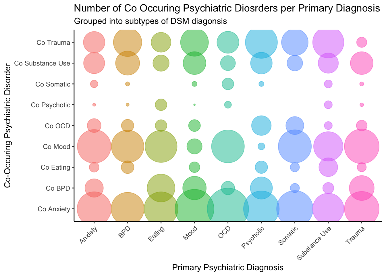
While very pretty, this visualization is hard to interpret as. It may
be easier to focus on the disorders most treated at the hospital (i.e.,
Anxiety, BPD, Mood, Trauma), and compare those across treatments.
I first wanted to find out the percentages of patients with one
diagnoses that also had another diagnosis. The following code: 1.
Creates a cross tabs of the number of people with each disorder / co
occuring disorders 2. Sums the number of people with a primary diagnosis
of anxiety, mood, trauma, and BPD 2. creates a value with the % of
people that also have co-occuring disorders.
Mothership_current_Imp <- Mothership %>%
  pivot_longer(
    cols=c(Anxiety_C, Mood_C, Substance_C, Trauma_C, BPD_Co_C,Other_Co,No_Co),
    names_to = 'Disorder_Present') %>%
  filter(value != 0) %>%
  select(!value)  %>%
  filter(!is.na(Disorder_Present))%>%
  filter(!is.na(Disorder_treat))


tabs<-as.data.frame.matrix(xtabs(~ Disorder_Present + Disorder_treat, data = Mothership_current_Imp))

anx<-summary(Mothership$Anxiety_D)[2]
bpd<-summary(Mothership$BPD_P)[2]
mood<-summary(Mothership$Mood_D)[2]
trauma<-summary(Mothership$Trauma_D)[2]

tabs[,1] <- (tabs[,1] / anx)*100
tabs[,2] <- (tabs[,2] /bpd)*100
tabs[,3] <- (tabs[,3] /mood)*100
tabs[,4] <- (tabs[,4] /trauma)*100

tabs[,5] <- c("Anxiety","BPD","Mood","None","Other","Substance","Trauma")
colnames(tabs)[5] = "Disorder"
tabs
##               Anxiety       BPD      Mood    Trauma  Disorder
## Anxiety_C   48.036649 56.727273 58.727001 45.418719   Anxiety
## BPD_Co_C    13.612565  0.000000 21.084038 23.054187       BPD
## Mood_C      46.727749 55.272727  8.577822 45.320197      Mood
## No_Co       15.575916  8.000000 19.194431 22.364532      None
## Other_Co     7.068063  6.545455  4.823471  3.546798     Other
## Substance_C 18.062827 29.818182 19.691696 19.113300 Substance
## Trauma_C    18.848168 41.818182 29.860766  3.645320    Trauma
Plot the thing
Now that we have the percentages we will need to plot it. This figure
plots the proportion of co-occuring disorders (y-axis) by the main
diagnoses treated (x axis).
Mothership_current_Imp %>%
ggplot(aes(x = Disorder_treat, y = Disorder_Present, color = Disorder_treat)) +
geom_count(aes(size = after_stat(prop),group = Disorder_treat), alpha = .75)+
scale_size_area(max_size = 40)+
scale_colour_manual(values = c("#FE6CAA","#f7a174","#B1D4E0","#A06CFE"))+
#scale_size_continuous(range = c(10, 30)) +
theme_classic() +
theme(axis.text.x = element_text(angle = 45,hjust = 1),
legend.position = "none") +
scale_y_discrete(labels=c("Other_Co" = "Other",
"No_Co" = "None",
"BPD_Co_C" = "BPD",
"Trauma_C" = "Trauma",
"Substance_C" = "Substance Use",
"Mood_C" = "Mood",
"Anxiety_C" = "Anxiety")) +
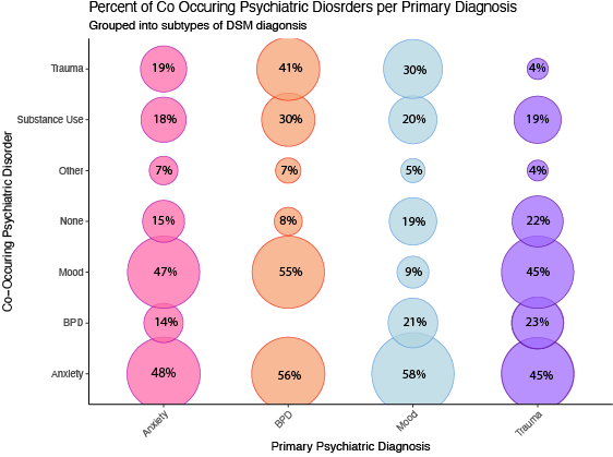
labs(title = "Percent of Co Occuring Psychiatric Diosrders per Primary Diagnosis",
subtitle = "Grouped into subtypes of DSM diagonsis",
y = "Co-Occuring Psychiatric Disorder",
x = "Primary Psychiatric Diagnosis")
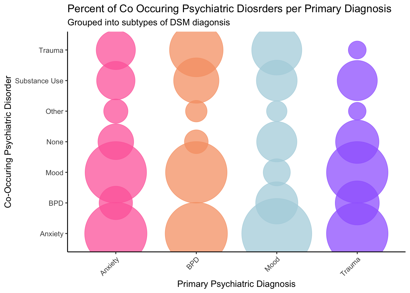
While this figure is more clear, I wanted to add numbers to it. I
popped this over to illustrator and made things a bit better. You can
see the final figure below:
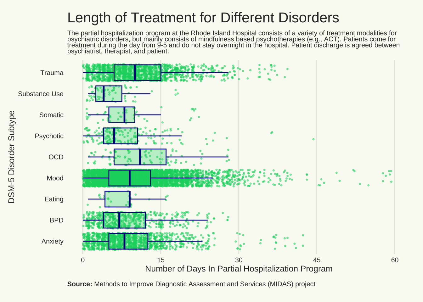
Duration of treatment based upon disorder
Source for Data_Vis
library(tidyverse)
#install.packages("showtext")
library(showtext)
# install.packages("camcorder")
library(camcorder)
# install.packages("ggtext")
library(ggtext)
library(glue)
# install.packages("nrbrand")
#require(nrBrand)
    #what the fuck is this?
# install.packages("ggmagnify")
#library(ggmagnify)


font_add_google("Fredericka the Great", "fred")
showtext_auto()

# gg_record(
#   dir = file.path("~/Desktop/Coding/R working directory/plots/Recording"), # where to save the recording
#   device = "png", # device to use to save images
#   width = 8, # width of saved image
#   height = 6.5, # height of saved image
#   units = "in", # units for width and height
#   dpi = 300 # dpi to use when saving image
# )


bg_col <- "#F9FBF2"
# highlight_col <- "#FFAD05"
# highlight_col <- "FF52825"
highlight_col <- "#02d46e"
outline_col <- "darkblue"
dark_col <- "#333333"

title = "Length of Treatment for Different Disorders"
st = "The partial hospitalization program at the Rhode Island Hospital consists of a variety of treatment modalities for psychiatric disorders, but mainly consists of mindfulness based psychotherapies (e.g., ACT). Patients come for treatment during the day from 9-5 and do not stay overnight in the hospital. Patient discharge is agreed between psychiatrist, therapist, and patient."

cap = "**Source:** Methods to Improve Diagnostic Assessment and Services (MIDAS) project <br> "

set.seed(12345)
ggplot(
  data = Mothership_Current_Long,
  mapping = aes(
    x = Days_complete_1,
    y = Disorder_Type,
    group = Disorder_Type)
  )+
  geom_jitter(
    size = 0.6,
    alpha = .5,
    colour = highlight_col
    )+
  geom_boxplot(
    outlier.shape = NA,
    colour = outline_col,
    fill = highlight_col,
    alpha = 0.3) +
  scale_x_continuous(
   breaks = c(0, 15, 30, 45, 60),
    limits = c(0.00, 60)
  ) +
  labs(
    x = "Number of Days In Partial Hospitalization Program",
    y = "DSM-5 Disorder Subtype",
    title = title,
    subtitle = st,
    caption = cap
    ) +
  theme_minimal(
    base_size = 10,
    base_family = "Commissioner"
    ) +
  theme(
    axis.ticks = element_blank(),
    panel.grid.minor = element_blank(),
    panel.grid.major.y = element_blank(),
    panel.grid.major.x = element_line(
       linewidth = 0.4,
       colour = alpha(dark_col, 0.2),
    ),
    plot.background = element_rect(
      fill = bg_col,
      colour = bg_col
    ),
    panel.background = element_rect(
      fill = bg_col,
      colour = bg_col
    ),
    plot.title = element_text(
      family = "Commissioner",
        #this is the font
      margin = margin(b = 10),
      colour = dark_col,
      size = 17
    ),
    plot.subtitle = element_textbox_simple(
      lineheight = 0.55,
      colour = dark_col,
      family = "Commissioner",
      hjust = 0,
      margin = margin(b = 10),
      halign = 0,
      size = 8
    ),
    plot.caption = element_textbox_simple(
      lineheight = 0.55,
      colour = dark_col,
      margin = margin(t = 10)
    ),
    axis.text = element_text(colour = dark_col),
    axis.title = element_text(colour = dark_col),
    legend.position = "none",
    plot.margin = margin(15, 15, 10, 10)
  )
CUXOS by Diagnosis
Code
# install.packages("ggridges")
library(ggridges)
library(ggplot2)
library(forcats)
bg_col <- "#F9FBF2"
dark_col <- "#333333"

title = "Baseline Anxiety for Patients By Disorder Type"
subtitle = "Upon entrence of the partial hospitalization program, scores of anxiety are reported from the _Clinically Useful Anxiety Outcome Scale_ (CUXOS). The CUXOS is a 20 item measure used to assess symptoms of anxiety; a cutoff score of 20 suggests a possitive screen for a probable anxiety disorder. Mean CUXOS scores are reported for each disorder type below (i.e., _the black line_)."
cap = "**Symptom severity:** 0-10 (non-anxiety), 11-20 (minimal anxiety), 21-30 (mild anxiety), 31-40 (moderate anxiety), 41+ (severe anxiety) <br> <br> **Source:**: Methods to Improve Diagnostic Assessment and Services (MIDAS) project"


p <- ggplot(Mothership_Current_Long, aes(
  x = BL_CUXOS,
  y = Disorder_Type,
  fill = Disorder_Type)) +
  # geom_density_ridges(alpha=0.6,
  #                     rel_min_height = 0.05,
  #                     scale = 2)+
   stat_density_ridges(quantile_lines = TRUE, alpha = 0.6, quantiles = 2, rel_min_height = 0.05, scale = 1.5) +
   scale_x_continuous(
   breaks = c(0, 20, 40, 60, 80),
   limits = c(0, 80)) +
  #theme_ridges() +
  labs(
    x = "Baseline Score on CUXOS",
    #y = "DSM-5 Disorder Subtype",
    title = title,
    subtitle = subtitle,
    caption = cap) +
   theme_minimal(
    base_size = 10,
    base_family = "Commissioner"
    ) +
    theme(legend.position = "none",
          axis.ticks = element_blank(),
    panel.grid.minor = element_blank(),
    panel.grid.major.y = element_blank(),
    panel.grid.major.x = element_line(
       linewidth = 0.4),
    axis.title.y= element_blank(),
    plot.background = element_rect(
      fill = bg_col,
      colour = bg_col
    ),
    panel.background = element_rect(
      fill = bg_col,
      colour = bg_col
    ),
    plot.title = element_text(
      family = "Commissioner",
        #this is the font
      margin = margin(b = 5),
      colour = dark_col,
      size = 15
    ),
    plot.subtitle = element_textbox_simple(
      lineheight = 0.55,
      colour = dark_col,
      family = "Commissioner",
      hjust = 0,
      margin = margin(b = 6),
      halign = 0,
      size = 8
    ),
     plot.caption = element_textbox_simple(
      lineheight = 0.55,
      colour = dark_col,
      margin = margin(t = 10),
      size = 7))
Plot
p

Depression by disorder type
Code
bg_col <- "#F9FBF2"
dark_col <- "#333333"
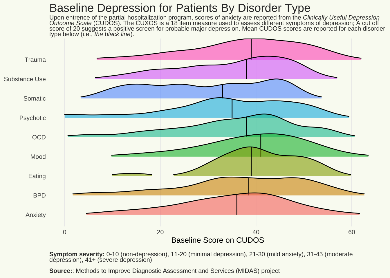
title = "Baseline Depression for Patients By Disorder Type"
subtitle = "Upon entrence of the partial hospitalization program, scores of anxiety are reported from the _Clinically Useful Depression Outcome Scale_ (CUDOS). The CUXOS is a 18 item measure used to assess different symptoms of depression; A cut off score of 20 suggests a positive screen for probable major depression. Mean CUDOS scores are reported for each disorder type below (i.e., _the black line_)."
cap = "**Symptom severity:** 0-10 (non-depression), 11-20 (minimal depression), 21-30 (mild anxiety), 31-45 (moderate depression), 41+ (severe depression) <br><br> **Source:**: Methods to Improve Diagnostic Assessment and Services (MIDAS) project"
q <- ggplot(Mothership_Current_Long, aes(
x = BL_CUDOS,
y = Disorder_Type,
fill = Disorder_Type)) +
# geom_density_ridges(alpha=0.6,
# rel_min_height = 0.05,
# scale = 2)+
stat_density_ridges(quantile_lines = TRUE, alpha = 0.6, quantiles = 2, rel_min_height = 0.05, scale = 1.5) +
scale_x_continuous(
breaks = c(0, 20, 40, 60),
limits = c(0, 64)) +
#theme_ridges() +
labs(
x = "Baseline Score on CUDOS",
#y = "DSM-5 Disorder Subtype",
title = title,
subtitle = subtitle,
caption = cap) +
theme_minimal(
base_size = 10,
base_family = "Commissioner"
) +
theme(legend.position = "none",
axis.ticks = element_blank(),
panel.grid.minor = element_blank(),
panel.grid.major.y = element_blank(),
panel.grid.major.x = element_line(
linewidth = 0.4),
axis.title.y= element_blank(),
plot.background = element_rect(
fill = bg_col,
colour = bg_col
),
panel.background = element_rect(
fill = bg_col,
colour = bg_col
),
plot.title = element_text(
family = "Commissioner",
#this is the font
margin = margin(b = 5),
colour = dark_col,
size = 15
),
plot.subtitle = element_textbox_simple(
lineheight = 0.55,
colour = dark_col,
family = "Commissioner",
hjust = 0,
margin = margin(b = 5),
halign = 0,
size = 8
),
plot.caption = element_textbox_simple(
lineheight = 0.55,
colour = dark_col,
margin = margin(t = 10),
size = 8))
plot
q